Q2 2026 Portfolio Commentary
A Long/Short Longboat Update


This commentary is based upon client portfolio performance reports.
It is intended as supplementary material to those reports.
You can access your client portal which includes these reports here:
Investing is a means to an end and is step 3 in our financial planning process.
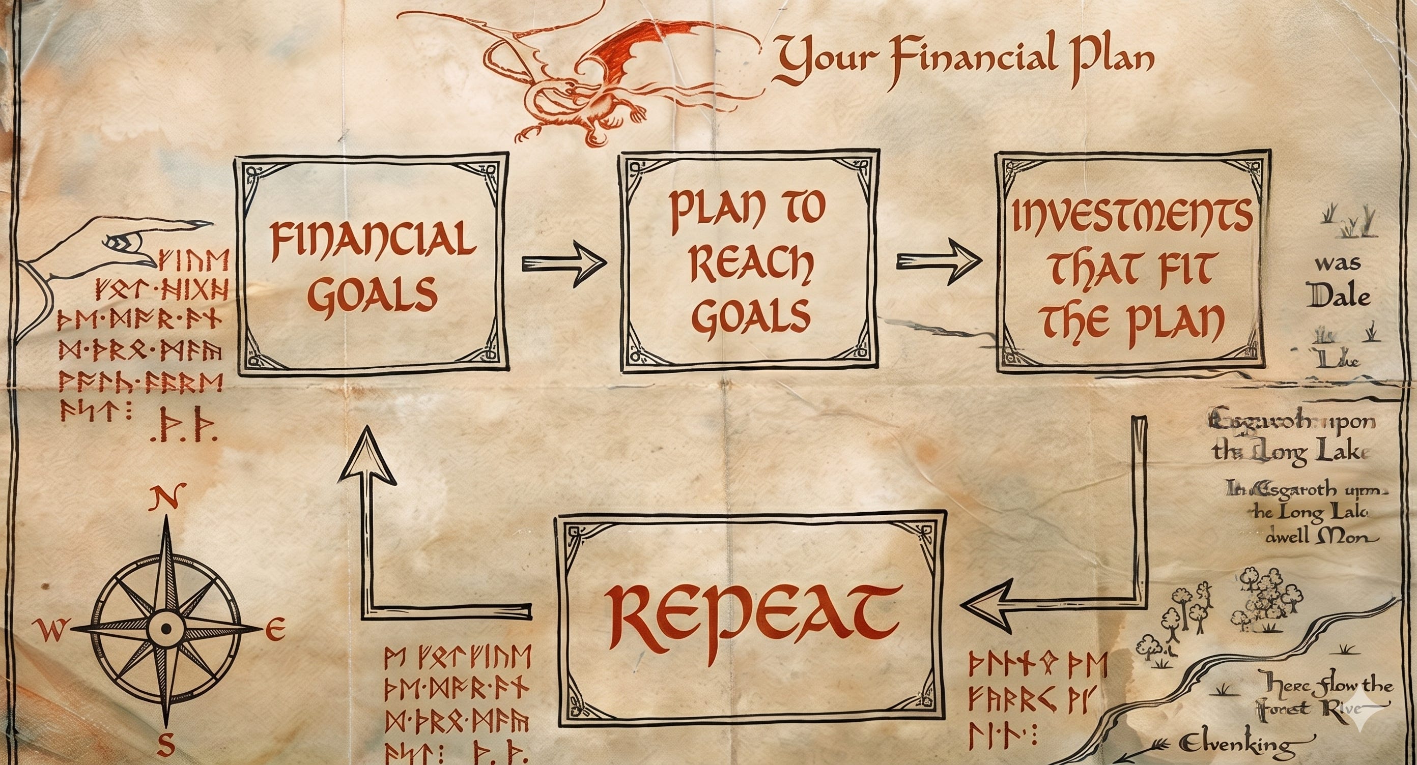
That end is accomplishing your financial goals per your custom financial plan.

Every financial plan relies on an implied required return (RR) that must be earned over the long term to remain robust.
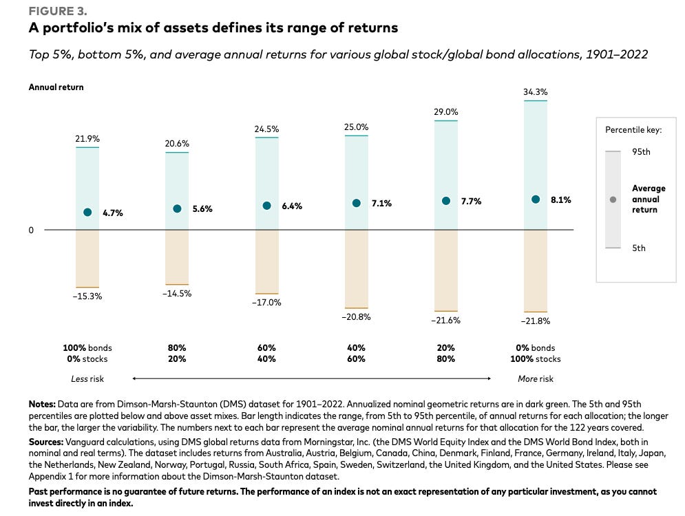
To help manage expectations, the following illustrates the historical range of annual returns (top 5%, bottom 5%, and average) for various global stock and bond allocations over 120+ years (1901–2022).
This range spans from the least risky allocation (100% bonds on the left) to the most risky (100% stocks on the right).
Now, let us compare the managed portfolios’ performance to their RR and comparable low-cost, publicly traded diversified benchmarks.

Aggressive Portfolios
They underperformed the Required Return (RR) benchmark for the quarter.
They underperformed the Comparable Portfolio Benchmark for the quarter.
Balanced Portfolios
They underperformed the Required Return (RR) benchmark for the quarter.
They underperformed the Comparable Portfolio Benchmark for for the quarter.
Cash Reserve Portfolios
They performed in line with the Required Return (RR) benchmark for the quarter.
They performed in line with the Comparable Portfolio Benchmark for the quarter.
The Equity Sleeve
It underperformed the benchmark for the quarter.
Contributors
High Quality US Large Companies, High Quality US Small Companies, and Semiconductors added value.
Detractors
US Large Companies + Managed Futures, Global Armaments, and Precious Metal Royalty Companies subtracted value.
Exited Positions
Bitcoin
Despite our long-term bullish view, we use a quantitative risk management process similar to commodity trading advisors (CTAs).
We fully exited in January thus avoided a double-digit drawdown before we began rebuilding the position in April.
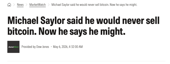
However, the risk system flashed a warning in May thus we exited at a low single-digit loss, preventing another significant drawdown.
We will likely re-establish exposure once conditions become favorable.
For our deep dive into this topic, checkout this post:

Bitcoin’s severe contraction was driven by physical constraints on the global electrical grid, ETF outflows, and the sword of leverage cutting both ways.
Electrical Grid Constraints
AI datacenter build-outs, legacy electrification, and North American LNG demand dismantled assumptions of cheap energy supporting Bitcoin.
Explosive growth in AI demand has driven tech giants to bid up electricity prices, rendering mining unprofitable.
To bypass grid bottlenecks, tech giants adopted on-site “behind-the-meter” Combined Cycle Gas Turbine generation for their own exclusive use.
Priced out by AI datacenters paying several times more per kilowatt, miners faced an existential crisis. With costs near $130,000 per coin against spot prices below $70,000, the deeply unprofitable industry forced exits, though some pivoted to AI compute.
ETF Outflows
Bitcoin’s 2024–2025 surge was helped by the “passive bid” via ETFs. Its price is highly reflexive and sensitive to marginal capital flows.
Historically, net ETF flows explained roughly 85% of Bitcoin’s price variance. Due to mining dilution, baseline inflows are necessary to sustain flat prices; without positive ETF inflows, Bitcoin’s price has a material headwind.
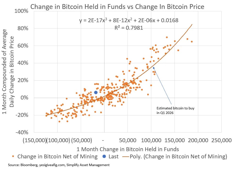
By Q2 2026, this passive bid evaporated as high interest rates and geopolitical uncertainty led investors to reduce high-beta risk exposure. Heavy US ETF net outflows in May and June 2026 mechanically forced fund sponsors to liquidate physical Bitcoin to cash out redeeming ETFs.
The sell-off was exacerbated by massive quarterly options expirations and systemic tax-loss harvesting.
The Sword of Leverage Cuts Both Ways
MicroStrategy served as a systemic point of failure due to its highly leveraged balance sheet. The firm became a Bitcoin treasury vehicle, accumulating over 250,000 Bitcoins via convertible debt and equity facilities.
This strategy utilized a reflexive loop: issuing debt to buy Bitcoin lifted prices, expanding its NAV and stock premium, which enabled further financing like a $3 billion 0.0% note in late 2024.
By mid-2026, a severe capital mismatch exposed this vulnerability. It had only $600 million to $700 million in cash (4 to 5 months of runway) against a $1.7 billion annual funding obligation, including $150 million monthly dividends for its preferred shares.
To meet liquidity needs, it controversially sold Bitcoin to pay dividends, violating public commitments and causing market panic. This structural selling created a “source of funds” discount, inducing rapid investor liquidations.
Sector ETFs
These exposures included:
US Energy Sector
US MLP and Energy Infrastructure Sector
US Utilities
US Basic Materials
Norwegian Energy
They gained Quantamental signal strength at the start of Gulf War 3.
When rolling ceasefires began, the signal rapidly reversed into negative territory, prompting us to exit the positions.

Semiconductors
Prior to Gulf War 3, this exposure had strong Quantamental signal strength.
Within a week, the Quantamentals for Semiconductors degraded materially, prompting us to exit the position.
When rolling ceasefires began, the signal quickly reversed into positive territory, prompting us to re-enter.
However, realizing that the rapid price rise was driven by massive levered global bets, we recognized that the dual-edged sword of highly levered trades cuts both ways.
We were not comfortable thinking we could exit in time to prevent the damage that might unfold at unprecedented speed.
That of course is in addition to the implied expectations in these semiconductor stocks.
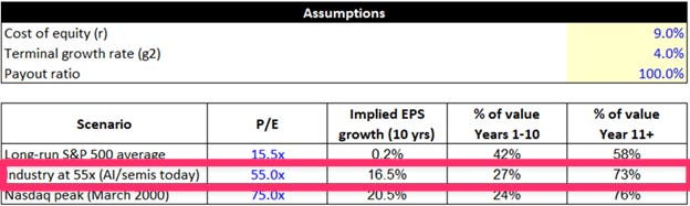
About 75% of the global semiconductor industry’s value relies on cash flow projections beyond 10 years. Yet, a decade ago, leaders like OpenAI and Anthropic did not exist. Future uncertainties include:
AI designing its own chips, accelerating obsolescence
Innovations bypassing current supply chain bottlenecks
Software reducing required compute for models
Chinese open-source models eroding US frontier advantages cheaply
While these specific scenarios may be unlikely, current market valuations dangerously assume certainty in rosy long-term forecasts precisely when actual uncertainty is highest.
As such, we exited the position.
High Quality US Large Companies
This exposure consists of US Large Companies and then seeks to earn superior long term returns with lower downside risk by filtering out junk companies (overvalued and low quality companies run by poor management teams).
While we still think this is an excellent way to gain exposure to High Quality US Large Companies, we concluded a better long term exposure is instead the stacking of two exposures on top of one another.
US Large Companies (the passive S&P 500 Index)
An uncorrelated alternative return strategy
We discuss this updated exposure in the new portfolio management tool and new position section.
Maintained Positions
Systematic Long/Short Extensions
This position only applies to those with large taxable account balances.
This takes tax loss harvesting 1.0 and upgrades it to tax loss harvesting 2.0.
It enhances after-tax wealth compounding within a risk-managed framework. Practical uses include diversifying concentrated stocks, revitalizing “frozen” taxable accounts with large unrealized capital gains, and accumulating capital losses to offset future gains and lower taxes.
For our deep dive into this topic, checkout this post:

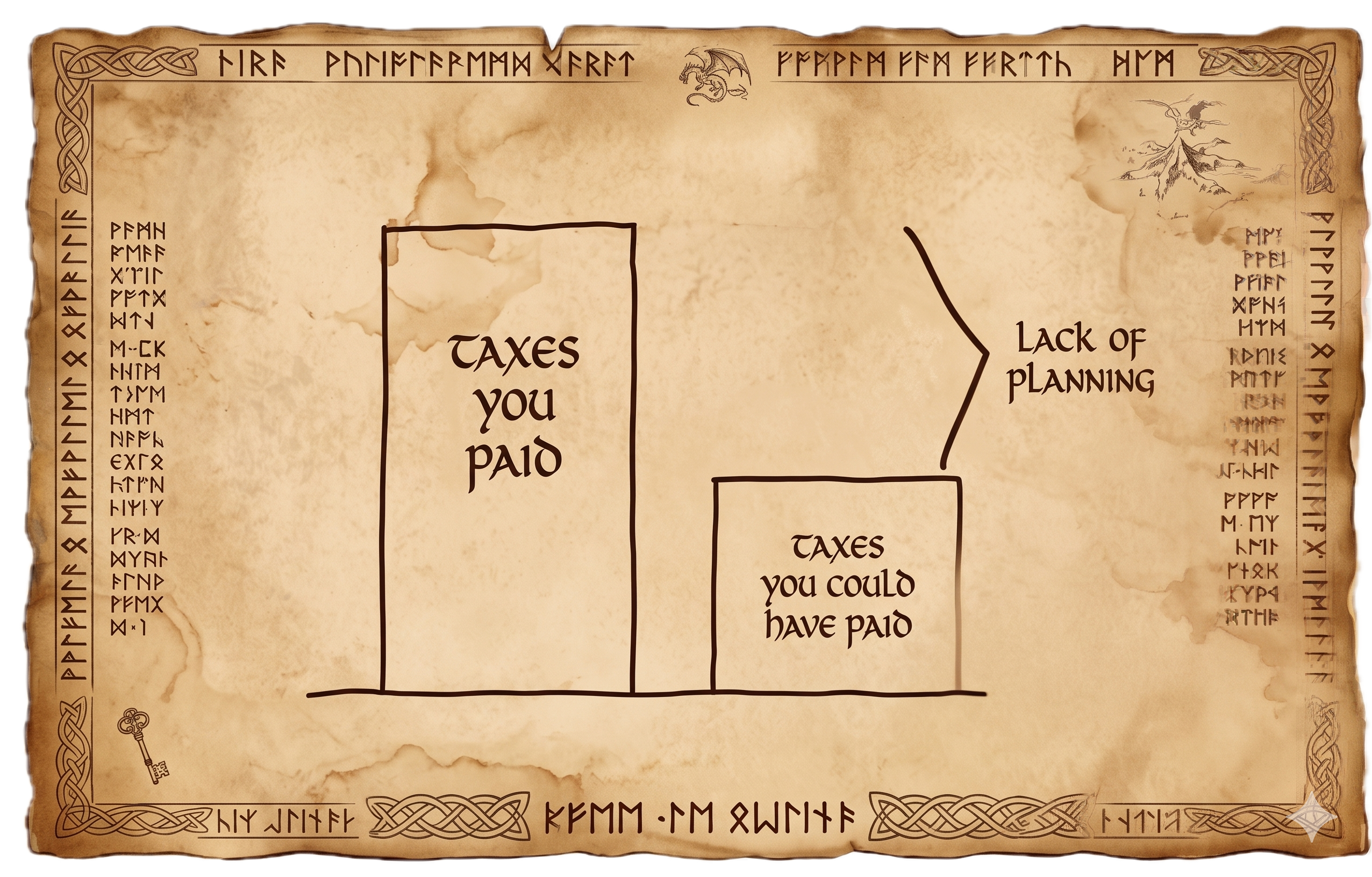
This is one of many tools we use for client tax planning.
It was in line with the benchmark for the quarter.
Moreover, reducing concentrated positions with significant embedded capital gains yielded only net short-term capital losses.
These capital losses were from closing both short and long positions, reflecting the quarter’s choppy equity market.
Going long means making money when prices rise.
This is buying low then selling high.
Going short means making money when prices fall.
This is selling high then buying low.
High Quality US Small Companies
This exposure consists of US Small Companies and then seeks to earn superior long term returns with lower downside risk by filtering out junk companies (overvalued and low quality companies run by poor management teams).
It reduces downside risk by filtering out::
High External Financing: Companies overly dependent on debt or issuing stock (like a farmer selling land to buy seeds).
Wealth Destroyers: Companies reinvesting cash at returns below their cost of capital (e.g., borrowing at 8% to earn 2%).
Value Traps: Companies with intrinsic value below book value (like a cheap house with a cracked foundation).
For Q2 2026, it lagged due to a lack of lower-quality “junk” names and stock selection in Technology and Industrials.
Most of the benchmark’s return came from large exposures to lower-quality “junk” names.
These short-lived junk runs are typical of bull markets. However, June signaled a reversal as quality leadership returned.
Global Armaments

This exposure focuses on companies that make armaments for nation state security.
In summary: the entire world is rapidly rearming off an extremely low base of defense spending.
This long term trend remains intact.
For our deep dive into this topic, checkout this post:

It underperformed the benchmark for the quarter.
Given the extraordinary positive returns from our initial position years ago, a correction in the exposure is not shocking.
This pullback stems from a confluence of temporary factors: European shipbuilding contract shifts, NATO diplomatic trade disputes, volatile Middle East ceasefire cycles, aggressive U.S. regulatory limits on shareholder payouts, and a domestic budget battle.
European Shipbuilding Contract Shifts
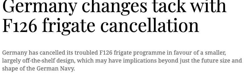
The European defense equity panic was triggered by Germany’s abrupt cancellation of its €10 billion F126 Niedersachsen-class frigate program. Originally awarded to Damen in 2020 for six anti-submarine warfare vessels, the project suffered chronic delays and cost overruns. When a proposed transfer to Rheinmetall’s Naval Vessels Lürssen (NVL) threatened to push total costs past €18 billion, Defense Minister Boris Pistorius canceled the program.
NATO Diplomatic Trade Disputes
In 2026, the European defense landscape faced severe disruption from NATO diplomatic and territorial disputes.
After a January U.S. military intervention in Venezuela—capturing leader Nicolás Maduro and seizing its oil reserves—defense equities initially surged.
However, the U.S. administration quickly pivoted to an aggressive push to acquire Greenland from Denmark, valuing its massive rare earth deposits and critical position for the “Golden Dome” missile defense shield.
Denmark and European allies responded by deploying over 200 troops to reinforce Greenland’s Joint Arctic Command. In retaliation, the U.S. enacted a 10% blanket tariff on allied goods on February 1, 2026, scheduled to rise to 25% on June 1 absent a deal.
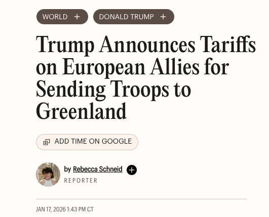
This move severely strained NATO relations, forcing institutional investors to reconsider transatlantic supply chain risks.
Volatile Middle East Ceasefire Cycles
Performance was heavily driven by a volatile sequence of Middle East ceasefires and re-escalations.
The 2026 US-Iran war disrupted global energy markets and sparked financial volatility.
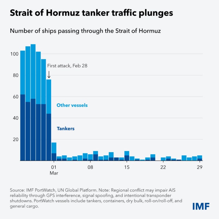
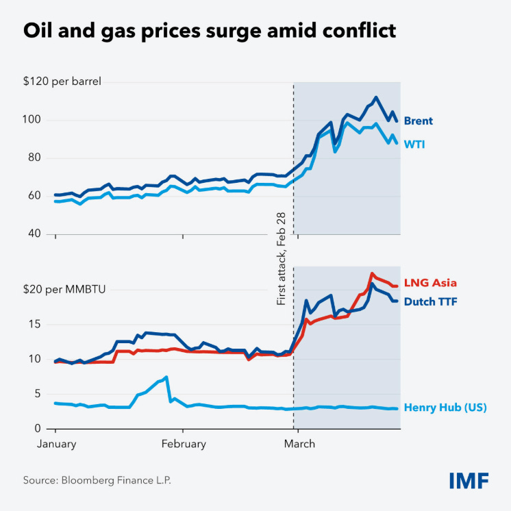
However, periodic negotiations yielded temporary diplomatic breakthroughs:
The April Ceasefire: Pakistan mediated an initial two-week truce on April 8, which President Trump extended indefinitely on April 21.
The Memorandum of (Mis)Understanding (MoMU): This 14-point pact established a 60-day negotiation window which eased the US blockade and oil sanctions in exchange for safe transit through the Strait of Hormuz.
This progress fostered a temporary “peace dividend” narrative in late June, prompting investors to rotate out of energy and defense holdings as Brent crude oil fell, US inflation cooled to 3.5%, and monetary easing expectations rose.
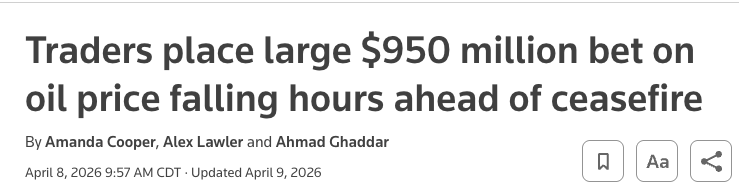
However, this optimistic period proved short-lived. On July 7, 2026, the truce collapsed when Iranian forces attacked commercial tankers, violating the MoMU.
President Trump terminated the agreement, resumed daily airstrikes against military targets inside Iran, and reinstated the naval blockade.
A proposed 20% security fee on Strait transit was quickly dropped due to allied backlash and energy cost concerns.
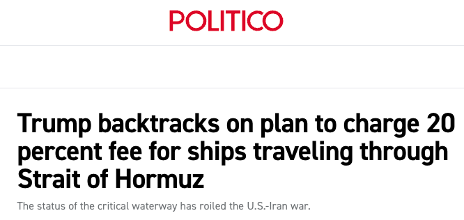
Renewed active hostilities and a 15% weekly surge in Brent crude collapsed the peace narrative, creating a highly volatile trading environment for defense assets.
US Regulatory Limits on Shareholder Payouts
Historically, a primary appeal of defense companies has been consistent free cash flow and capital returns via buybacks and dividends. Since 2020, the five largest contractors have spent over $100 billion on buybacks and dividends.
This model faced fierce criticism from the White House, who argue defense contractors prioritize profits and executive pay over industrial capacity and military readiness.
As such, Executive Order 14372 (”Prioritizing the Warfighter”) was issued on January 7, 2026. It directs the Secretary of Defense to restrict buybacks, dividends, and executive incentives for contractors underperforming or missing timelines on critical weapon systems.
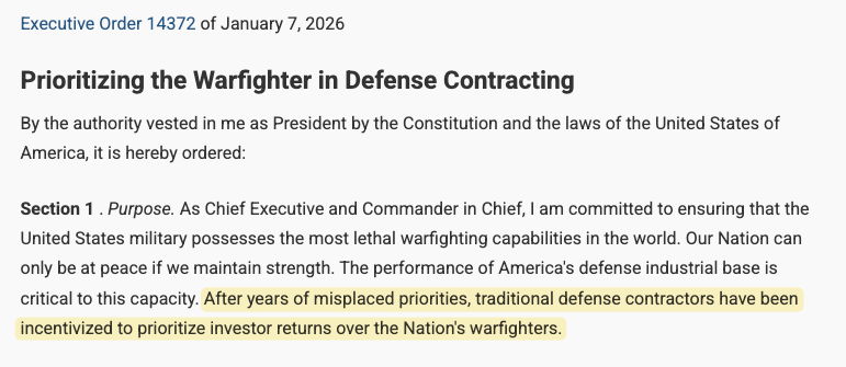
Consequently, threatened capital restrictions have introduced a structural valuation discount. Barring defense companies from returning cash to shareholders raises the sector’s cost of capital, reducing institutional appeal and depressing valuations across the entire complex.
Domestic Budget Battle
This domestic budget battle and policy scrutiny also contributed to the near-term volatility in defense companies.
In March 2026, the Pentagon requested $200 billion in emergency funds for Operation Epic Fury. Added to the $800 billion+ base budget, this constituted 20% to 25% of total 2026 military spending.
Progressive Democrats opposed funding the prolonged conflict, while fiscal hawks like Senator Joni Ernst demanded strict clarity on procurement and supply chain accountability.
Due to gridlock, lawmakers moved to fold defense funding into a broader reconciliation package. This compressed the projected defense portion from $200 billion down to $67–$72 billion by mid-July 2026.
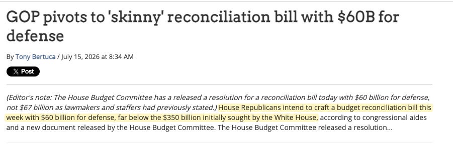
While defense spending growth remains positive long-term, this political friction caused near-term volatility and a valuation reset in 2026 as investors wait for promises to convert into audited corporate backlogs.
Japan (Dynamic Currency Hedging)

Filtering thru 1,300+ Japanese companies, this exposure excludes those with poor corporate governance and low shareholder yield (dividends or buybacks). The final portfolio contains fewer than 200 companies that statistically treat shareholders better than the unfiltered index.
Furthermore, the position dynamically hedges currency risk using four submodels to determine a hedge ratio from 0% (full Yen exposure) to 100% (no Yen exposure).
Foreign Investing 101
US investors buying Japanese stocks are affected by both the stock’s performance in Yen (local return) and the USD/Yen exchange rate (currency return).
Total Return = Local Stock Return + Currency Return
For our deep dive into this topic, checkout this post:

It underperformed the benchmark for the quarter.
Given the extraordinary positive returns from our initial position years ago, a correction in the exposure is not shocking.
The Q2 2026 lag is a tactical, mid-cycle consolidation caused by transient events: a historic central bank rate hike, a global tech sell-off, and geopolitical energy price spikes.
A Historic Central Bank Rate Hike
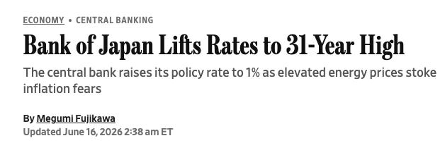
The Bank of Japan raised its policy rate to 1.00%, pushing borrowing costs to their highest since 1995 and ending ultra-loose monetary policy. This tightening triggered valuation compression on stocks, corporate borrowing concerns, capital outflows from real estate, and raised the 10-year JGB yield to levels last seen in 1996.
A Global Tech Sell-Off
A global tech and semiconductor sell-off occurred in June and July as investors questioned high AI capital expenditure valuations, prompting profit-taking that impacted Japanese hardware and chip-testing firms.
Geopolitical Energy Price Spikes
Middle East tensions renewed hostilities and drove Brent crude oil above $86 a barrel, increasing input costs for resource-importing Japan.
Precious Metal Royalty/Streaming Companies

This provides diversified precious metals (gold and silver) exposure, benefiting from price appreciation and mine production growth without operational mining risks.
The long-term thesis for precious metal royalty exposures remains intact, as precious metals continue to hedge against fiat currency debasement and systemic sovereign debt expansion.
For our deep dive into this topic, checkout this post:

It underperformed the benchmark for the quarter.
Given the extraordinary positive returns from our initial position years ago, a correction in the exposure is not shocking.
This pullback stems from a confluence of temporary factors: localized geopolitical liquidity shocks, a monetary regime shift at the Federal Reserve, and physical input bottlenecks in the global mining supply chain.
Localized Geopolitical Liquidity Shocks
The early 2026 precious metals sell-off was catalyzed by Gulf War 3 involving the US, Israel, and Iran. While Middle East conflicts typically spur safe-haven gold buying, this war triggered an unconventional, localized liquidity squeeze.
Historically major gold buyers, Middle Eastern countries faced depleted revenues as infrastructure bombardment and closed maritime routes compromised oil and gas exports. Strained by military financing and domestic subsidies, these actors abruptly halted gold accumulation.
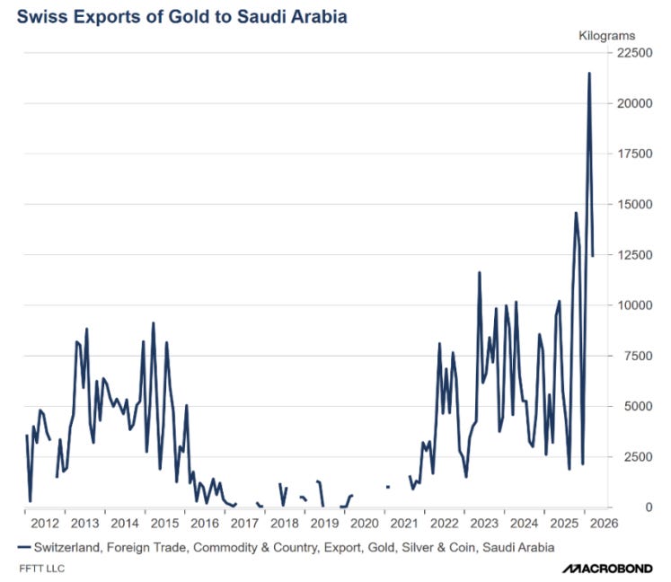
This pivot drove large-scale gold reserve liquidations.
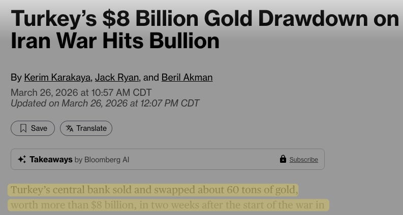
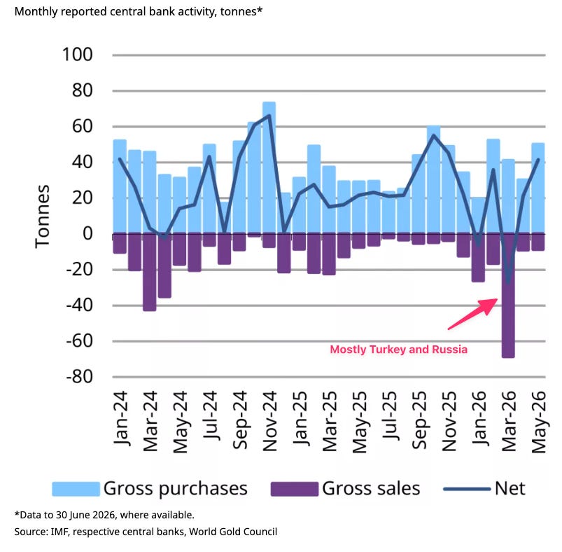
In Q2 2026, Turkey sold a substantial amount of gold reserves to defend its domestic currency from collapse, while Russia and other Gulf states liquidated gold holdings to fund spending demands.
This sudden supply shock overwhelmed commercial demand, depressing prices and causing one of the sharpest quarterly drawdowns for precious metals in thirteen years.
Monetary Regime Shift at the Federal Reserve
This geopolitical liquidity drain coincided with a historic leadership transition at the US Federal Reserve.
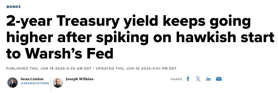
Kevin Warsh was sworn in as the 17th Chair, succeeding Jerome Powell. Defying market consensus anticipating a dovish shift for rate cuts, he declared “inflation is a choice” and asserted a resolute commitment to returning inflation to its strict 2% target, refusing to declare victory despite cooling consumer price index data.
The financial system’s response was swift: the 2-year US Treasury yield surged 16 basis points in a single day—the largest move on a Fed meeting day since March 2008—while the US Dollar Index strengthened significantly.
This tightening of global liquidity and rising volatility forced highly levered funds to execute systematic de-grossing procedures under strict risk mandates, liquidating their most liquid, profitable long positions.
Precious metals and precious metal equities, a primary source of prior institutional outperformance, became prime targets for a highly correlated market-wide liquidation.
Physical Input Bottlenecks
A physical supply-chain bottleneck compressed mining equity valuations and future stream expectations.
Sulfuric acid is indispensable for heap leaching desired metals from raw ore.
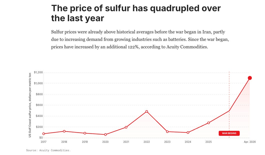
Gulf War 3 maritime disruptions closed the Strait of Hormuz, halting about 50% of the global seaborne sulfur trade used for sulfuric acid manufacturing. This shock intensified when China banned sulfuric acid exports to prioritize its domestic reserves.
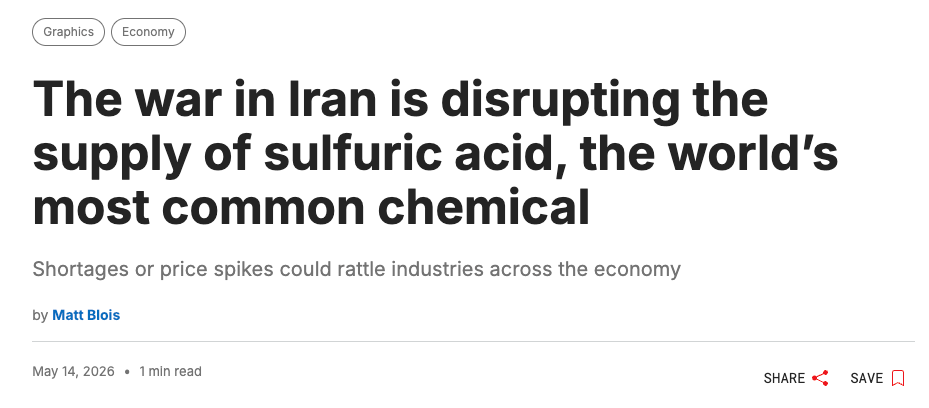
Consequently, spot sulfuric acid prices doubled in Chile, Peru, and the Democratic Republic of the Congo. Spot-market buyers faced immediate margin compression, and major miners like Anglo American downgraded their 2026 production guidance.
While royalty and streaming companies lack direct operating costs, their valuations depend on partner mines’ future volumes. Chemical shortages, delays, or guidance downgrades triggers equity markets to discount future royalty stream deliveries thus depressing stock prices.
West Texas Real Estate + Mineral Rights

This is West Texas Real Estate along with the associated oil, gas, and water rights.
Its long-term investment case remains intact, supported by five pillars: capital allocation compounding, high-margin royalties, stable water cash flows, contract-driven inflation protection, and emerging roles in AI infrastructure and alternative energy.
It underperformed the benchmark for the quarter.
Given the extraordinary positive returns from our initial position years ago, a correction in the exposure is not shocking.
Its Q2 2026 lag was driven by two catalysts: a global crude oil price reversal and a key board member’s unexpected passing.
A Global Crude Oil Price Reversal
In Q2 2026, it faced major macroeconomic headwinds from a sharp drop in global crude oil benchmarks.
Initially, Gulf War 3 caused West Texas Intermediate (WTI) crude to hit a multi year high of $112.84 per barrel.
This geopolitical risk premium dissolved after the signing of the 60-day Memorandum of (Mis)Understanding.
Then, a supply-side factor hit when the UAE left OPEC to aggressively capture market share.
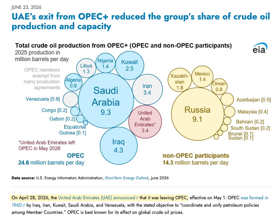
Consequently, WTI crude oil dropped around 30%.
Since its royalty revenues depend directly on energy prices, this commodity deflation lowered near-term top-line expectations and sparked sector-wide profit-taking.
A Key Board Member’s Unexpected Passing
It faced a governance shock when Board Member Murray Stahl unexpectedly died. As co-founder, CEO, and Chairman of Horizon Kinetics—its top institutional shareholder—he beneficially owned over 10 million shares (around 14.5% of outstanding common stock).
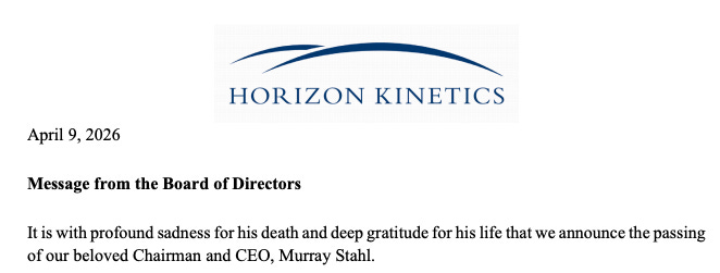
It fell shortly after since investors worried that management at Horizon Kinetics might liquidate its massive, highly concentrated position, creating long-term downward pressure.
To ensure continuity, the Board appointed Horizon Kinetics Co-Founder and Co-CEO Peter Doyle to the board. He joined pledged to maintain Stahl’s long-term investment philosophy and position.
New Portfolio Management Tool
Return Stacking
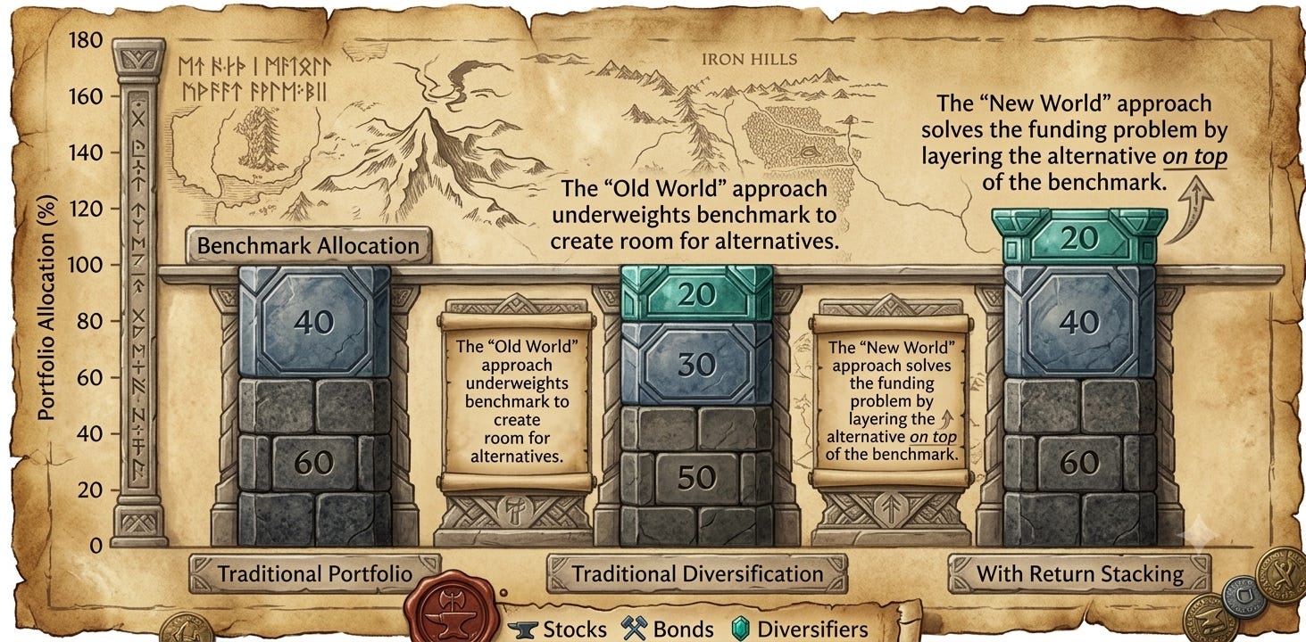
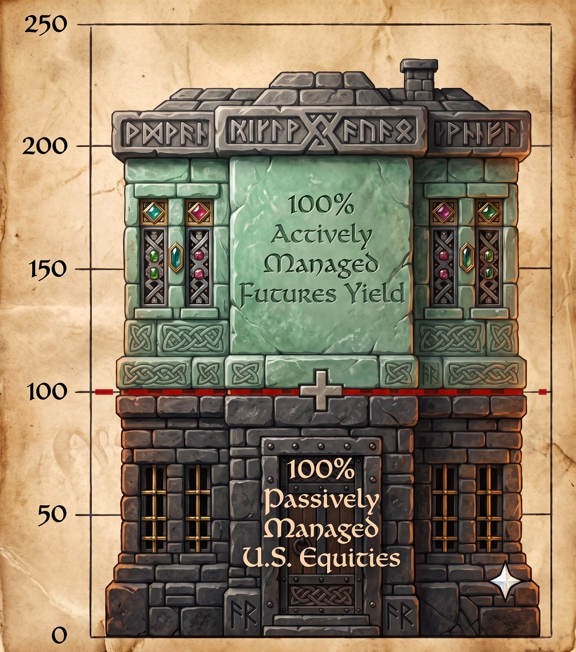
This portfolio management technique layers a diversifying investment on top of a core holding (like US Equities), achieving $2 of exposure per $1 invested.
Traditionally, adding diversifying alternatives (like managed futures, futures yield, merger arbitrage, or gold) required reducing the core holding.
Return stacking uses capital-efficient instruments to provide 100% exposure to the core holding and 100% exposure to alternatives simultaneously.
Think of it like adding a room to your house:
A traditional portfolio is a single-story house. To add a new office (alternatives), you must demolish your garage (sell core holding) to make room.
Return stacking builds a second story. You use capital-efficient engineering to layer the new room directly on top, keeping your entire ground floor (the core holding) intact.
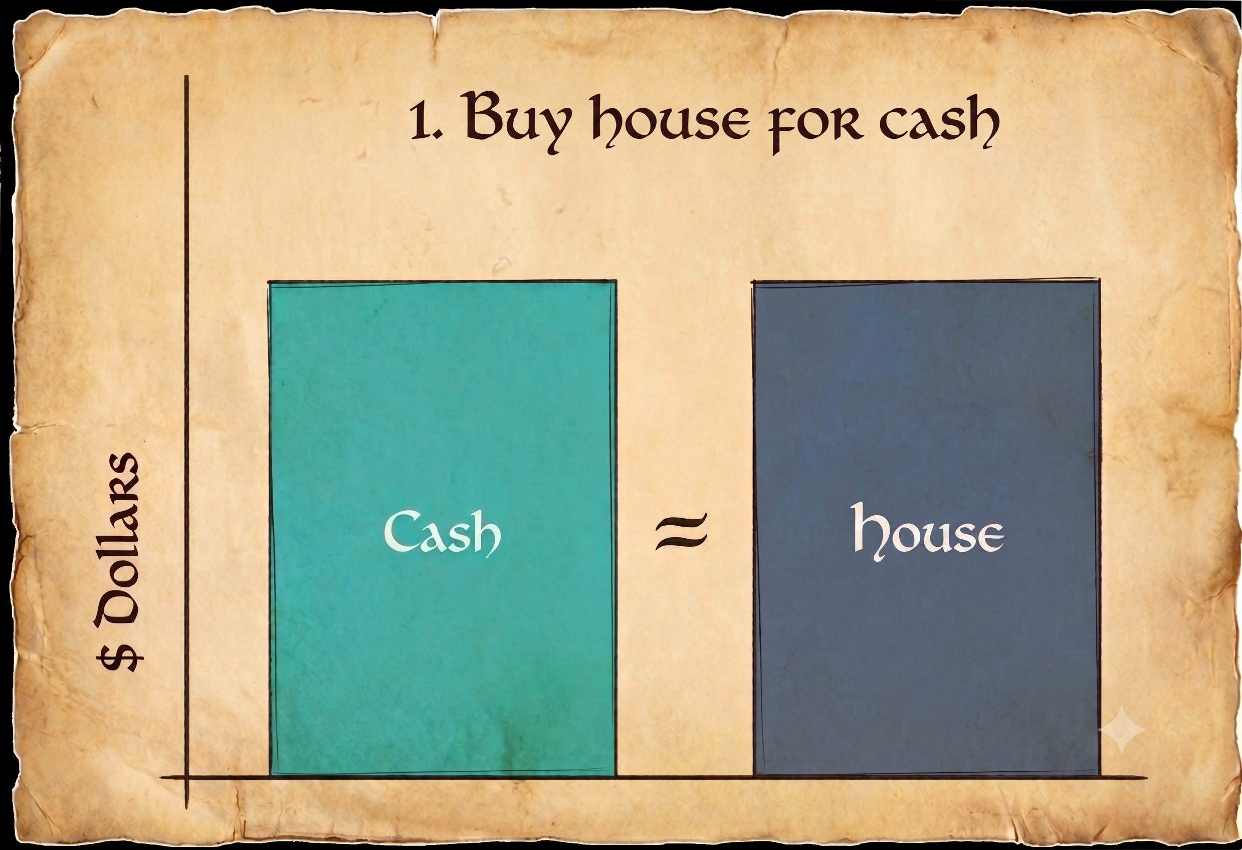
If You Bought A House, You Already Understand Return Stacking
Imagine buying a house outright with cash.
This means your return equals its appreciation or depreciation.
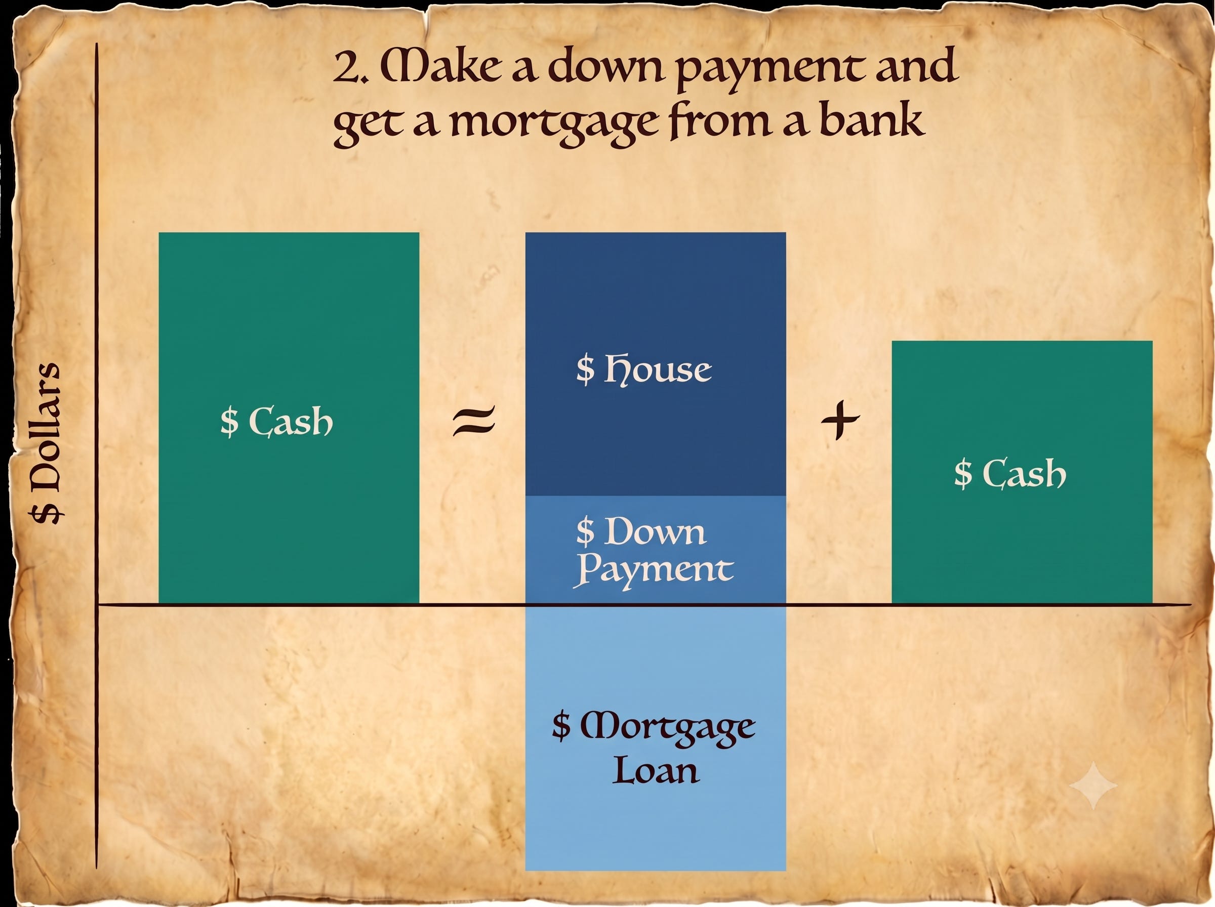
But what if instead of using all your cash, you take out a mortgage as well.
Why?
Because it allows you to leverage your money for more opportunities.
A smaller down payment and a mortgage allow you to own the house while keeping most of your cash.
This means your return equals the house’s appreciation or depreciation minus the mortgage’s interest costs.
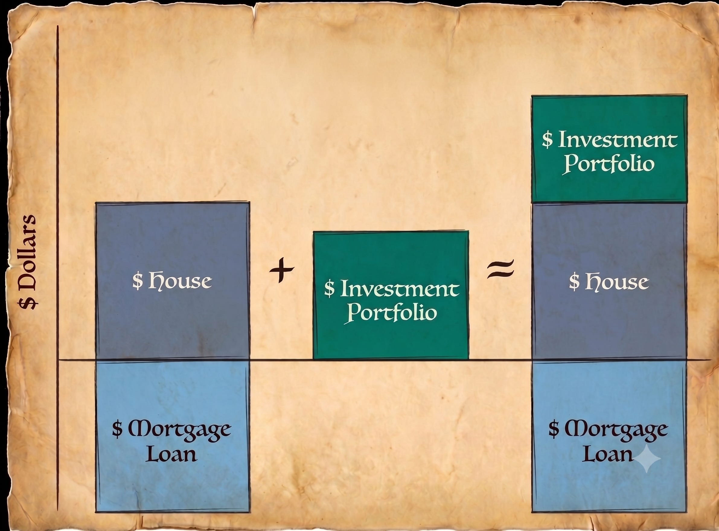
But what if you choose to invest your leftover cash elsewhere, effectively “stacking” an investment.
Why?
Because it allows you to combine home appreciation and investment returns, minus mortgage costs, potentially putting you in a better financial position than buying the house outright.
Moreover, if your investments rise during a real estate dip, you gain valuable diversification.
Instead of buying a home with a mortgage, we buy financial assets like stocks and bonds.
We borrow from institutional markets at rates close to short-term US Treasury Bills, which are often 2–3% cheaper than regular mortgage rates.
As before, the freed cash can be reinvested in various strategies to stack returns on top of existing stocks and bonds.
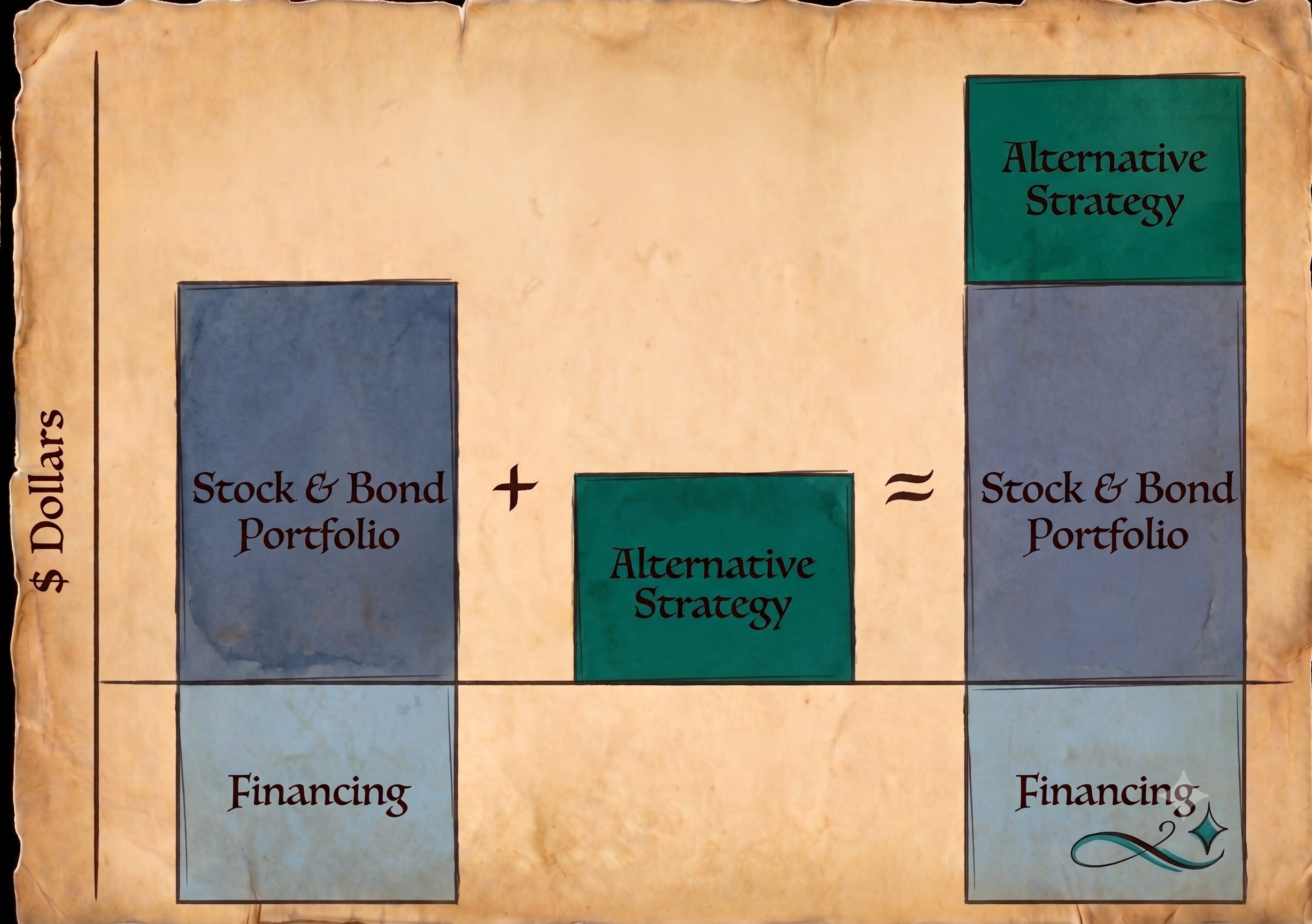
This changes the portfolio decision between the core holding and alternatives from “either-or” to “yes, and”.
In the past, we used the “either-or” approach because industry “yes, and” solutions were operationally difficult, expensive, and fragile.
Recent ETF innovations, SEC rule changes, and a single manager combining the core holding (1st floor) with an alternative strategy (2nd floor: managed futures, futures yield, gold, etc.) within one ETF represented a material improvement worth considering.
SEC Rule 18f-4
Before the SEC adopted Rule 18f-4 in February 2021, mutual funds and ETFs lacked clear guidance on derivative use. The rule now provides clear risk parameters for asset managers.
Combining your 1st floor (core holding) and 2nd floor (managed futures, futures yield, gold, etc.) exposures under one manager enables real-time, dynamic rebalancing—vital in volatile markets like Gulf War 3.
Thus this new portfolio management tool has been deployed across the managed portfolios.
Fun Fact
Delta Air Lines’ turnaround of its defined-benefit pension plan—from a precarious 35% funded status in 2011 to over 100%—is a landmark institutional finance case study in the use of “return stacking”.
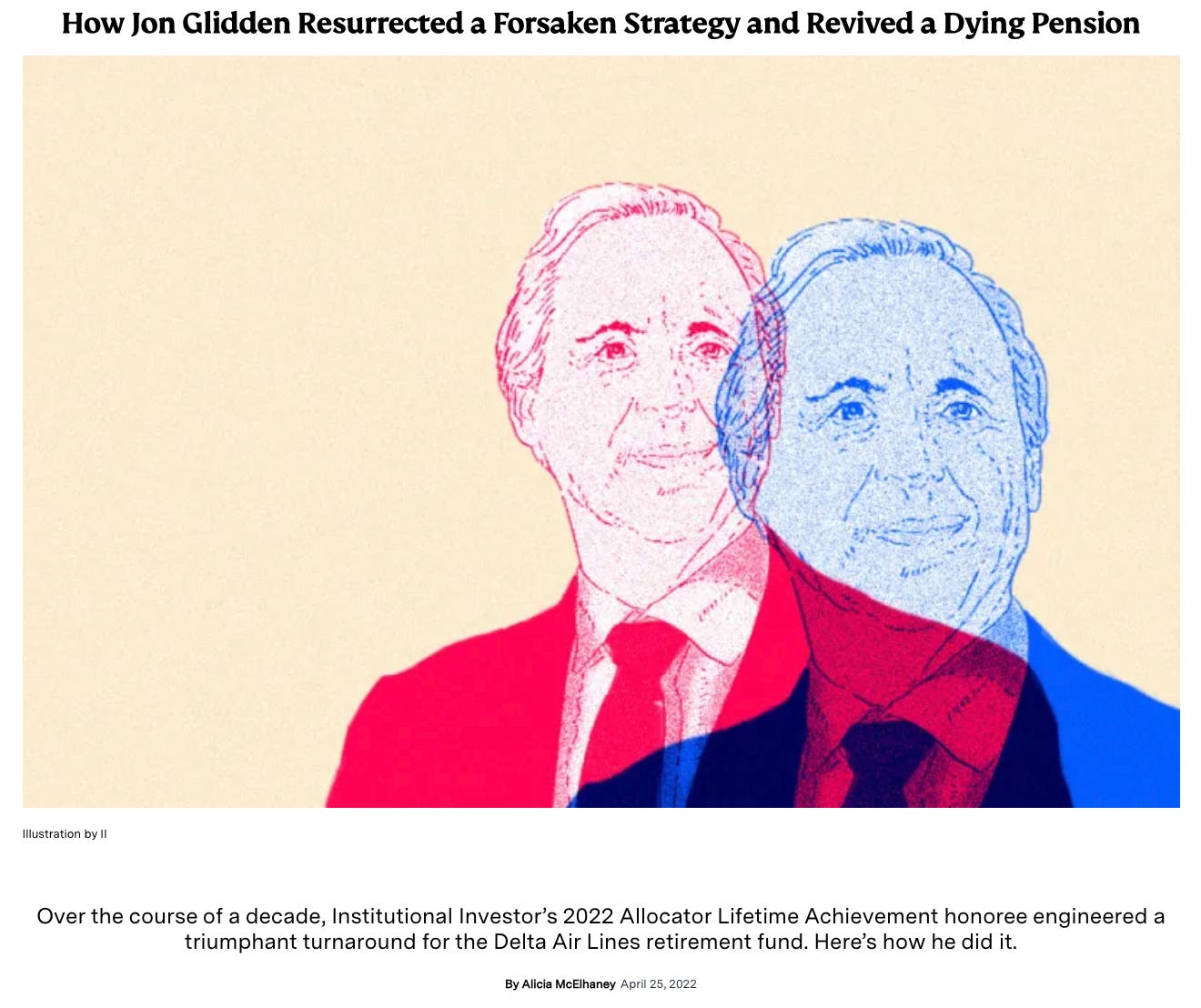
Traditionally called “Portable Alpha” by institutional investors, modern asset managers often use the term “Return Stacking” for the same concept: using capital-efficient derivatives for market exposure (beta) and stacking uncorrelated active strategies (alpha) on top.
New Positions
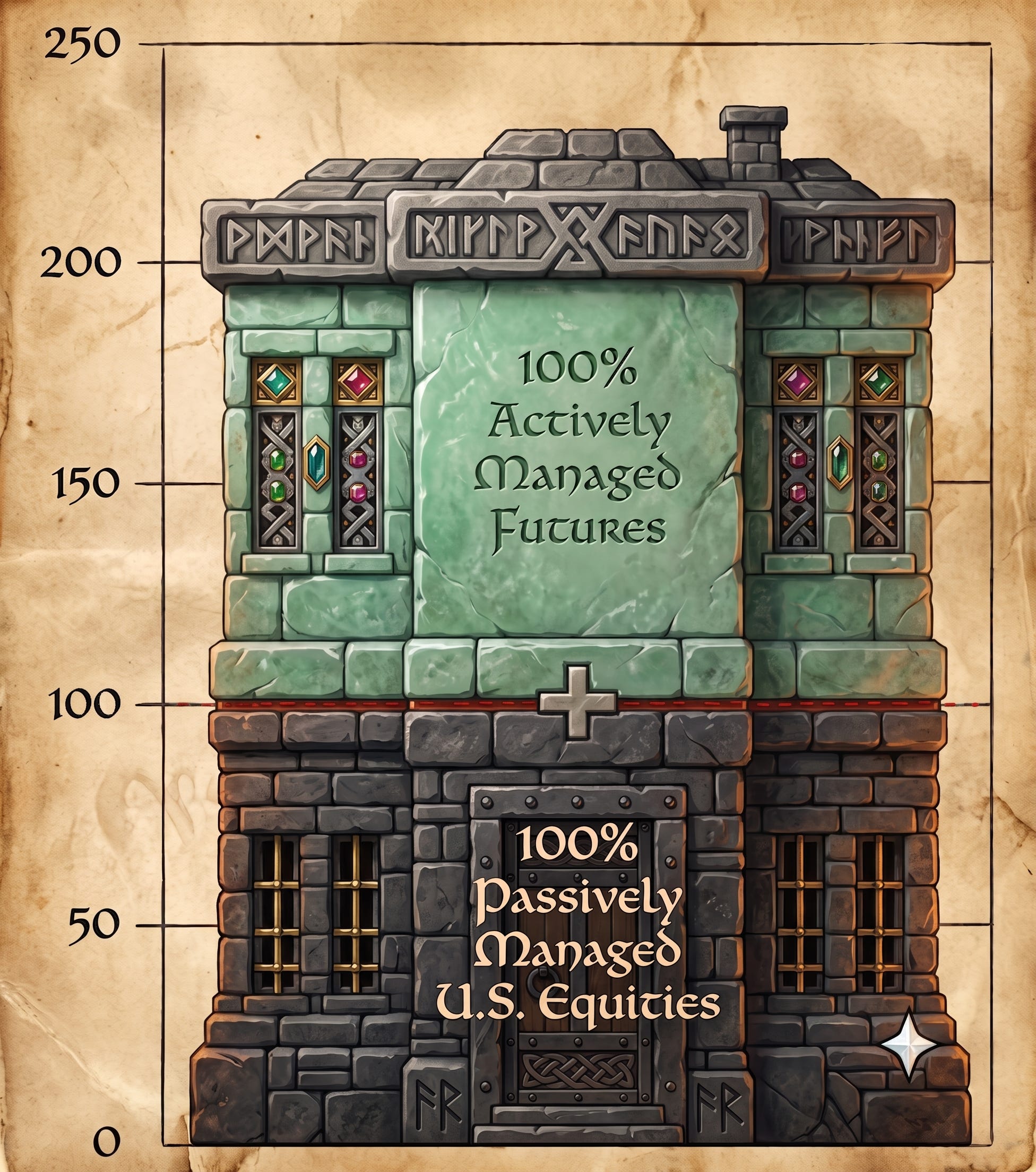
Passively Managed US Large Equities + Actively Managed Futures
The “1st story” is the S&P 500 which is the preeminent passive US Large Cap Equity index.
The “2nd story” is an actively managed futures strategy run by a current manager, with details in the alternatives section.
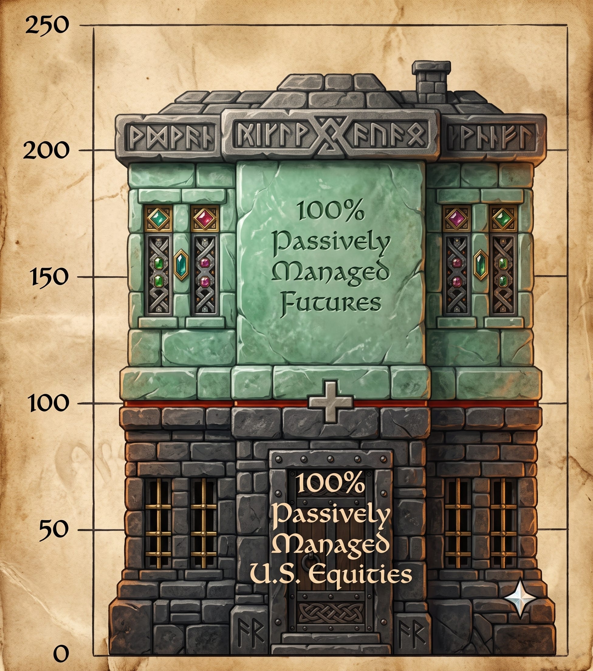
Passively Managed US Large Equities + Passively Managed Futures
The “1st story” layer is the S&P 500 which is the preeminent passive US Large Cap Equity index.
The “2nd story” layer is a passively managed futures strategy replicating the managed futures index. Details are covered in the alternatives section.
Passively Managed US Large Equities + Actively Managed Futures Yield
The “1st story” layer is the S&P 500 which is the preeminent passive US Large Cap Equity index.
The “2nd story” layer is an actively managed futures yield strategy. Details are covered in the alternatives section.
The Alternative Sleeve
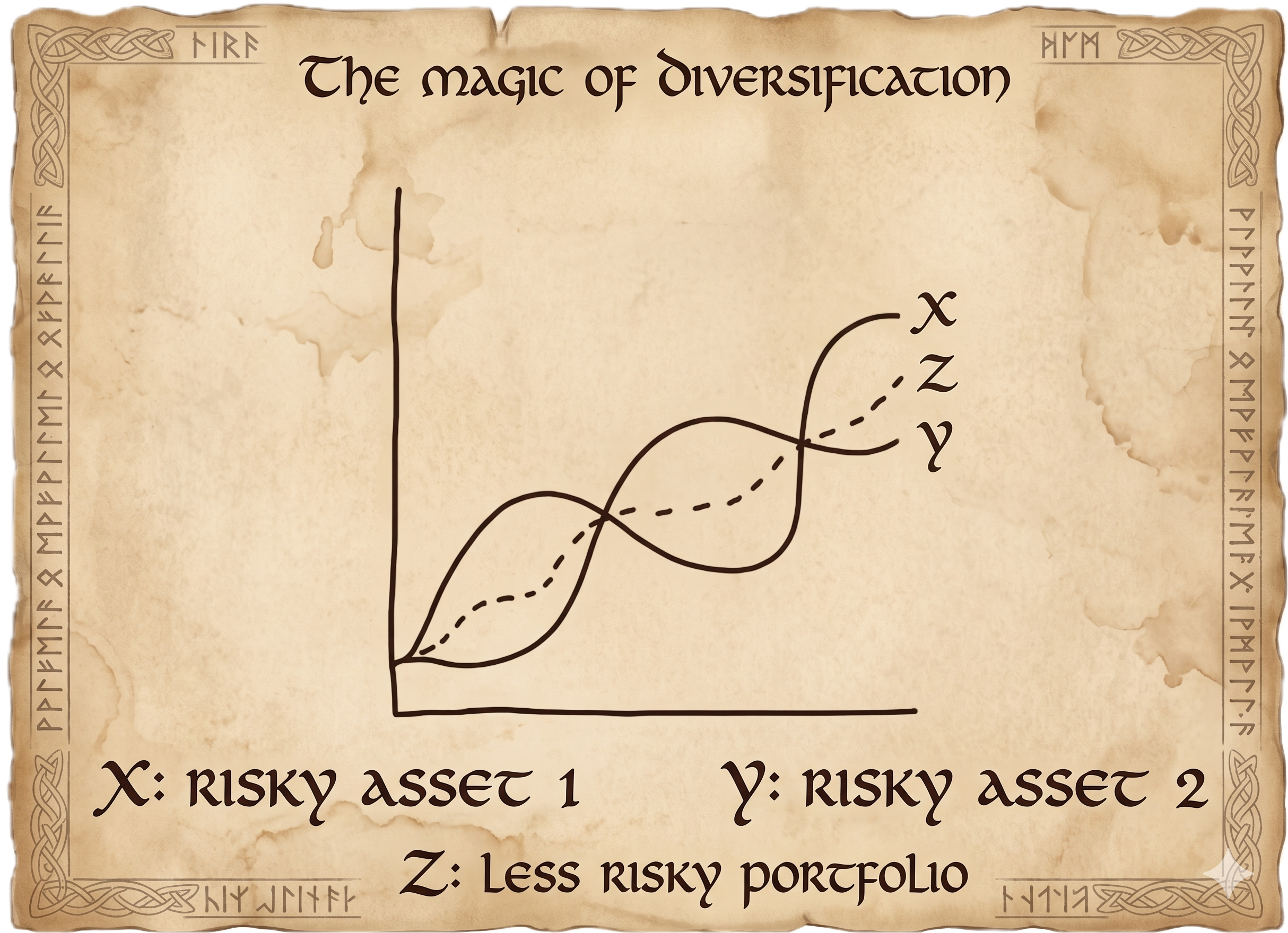
Our alternatives are designed for long-term absolute returns with low/negative correlation to equities, bonds, and other alternative strategies.
They zig when others zag.
It underperformed the benchmark for the quarter.
Contributors
Actively Managed Foreign Exchange (FX) added value.
Detractors
Actively Managed Futures and Fully Allocated Physical Gold Bullion subtracted value.
Exited Positions
Gresham’s Wrath (Gold Bullion with Income)
This exposure is a magnified gold exposure that also generates income.
We exited the position as the manager had changed the income generation strategy.
Previously, they generated income akin to selling a two-week fire insurance policy for $10 and buying reinsurance for $1, pocketing $9. This approach capped downside.
However, the manager shifted to something akin to selling fire reinsurance, removing the capped downside—a feature we considered essential.
Consequently, we exited the position.
Maintained Positions
Actively Managed Futures

This actively managed exposure seeks long-term absolute returns with low/negative correlation to equities, bonds, and other alternative strategies with downside protection during risk-off events.
It is a highly sophisticated form of trend following.
The long-term merit of this strategy (active or passive) stems from the human tendency to under-react to fundamental change by assuming the recent past will continue.
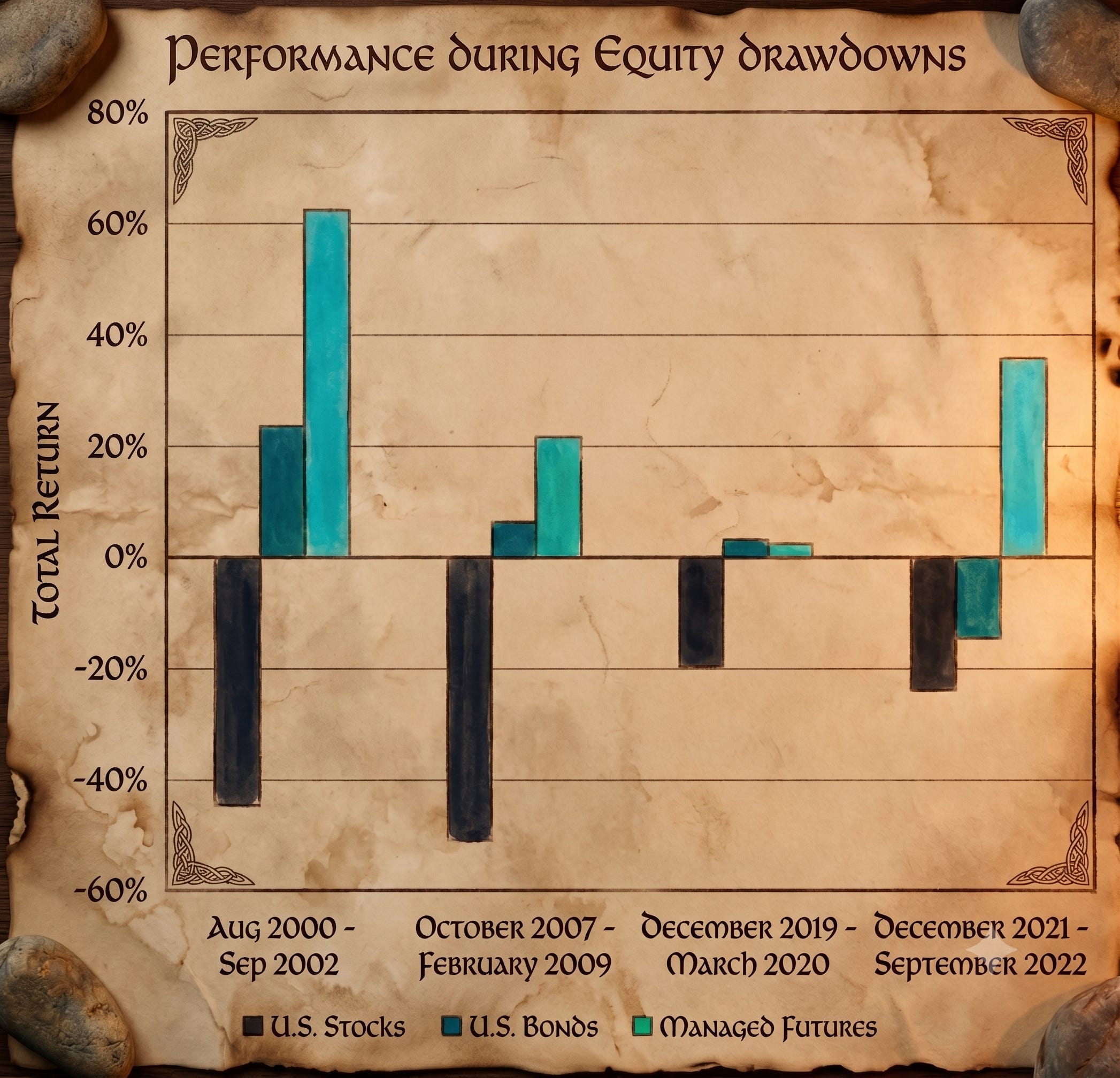
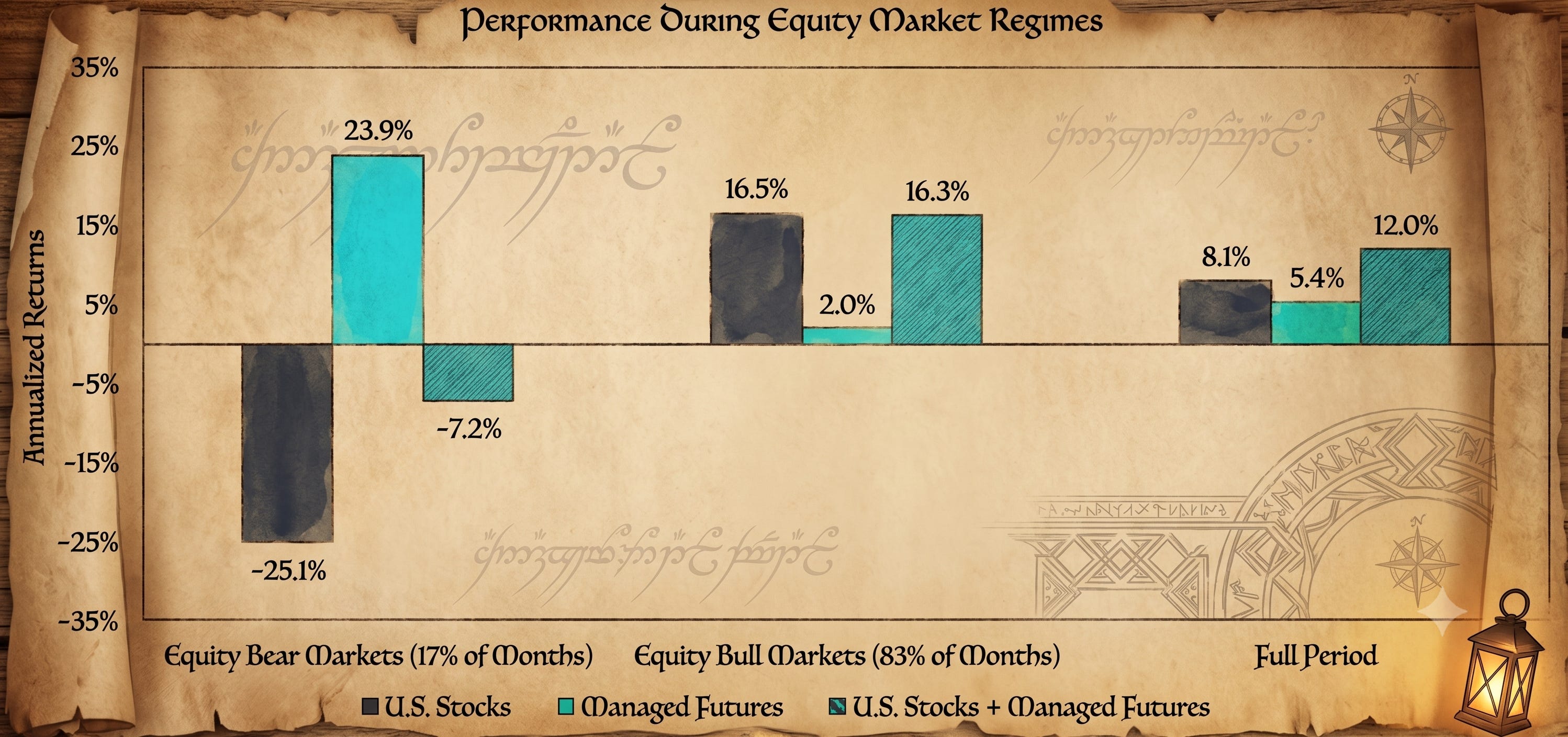
Below, the passive managed futures index shows its potency during equity drawdowns.
This managed futures exposure is now the “2nd floor” strategy that sits atop our “1st floor” S&P 500 strategy, the preeminent passive US Large Cap Equity index.
Thus, holding this alternative exposure does not reduce our equity exposure, which is important since equities are typically in an upward bull market.
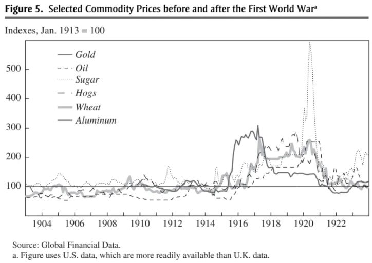
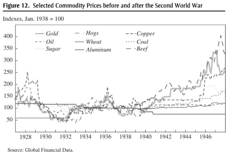
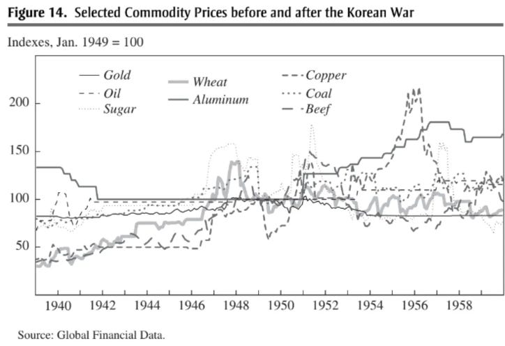
Applied History Break
For context, managed futures strategies significantly protected our capital in 2022 when most traditional stock and bond investors suffered heavy losses.
These strategies offer asymmetric value, especially at ultra-low armament spending starting points, leading to:
Failed deterrence and then;
Rising armament spending which disrupts bond markets and then;
Kinetic conflict which disrupts commodity markets.
We identified this pattern in our global armaments deep dive:
Given the extraordinary positive returns from our initial position years ago, a correction in the exposure is not shocking.
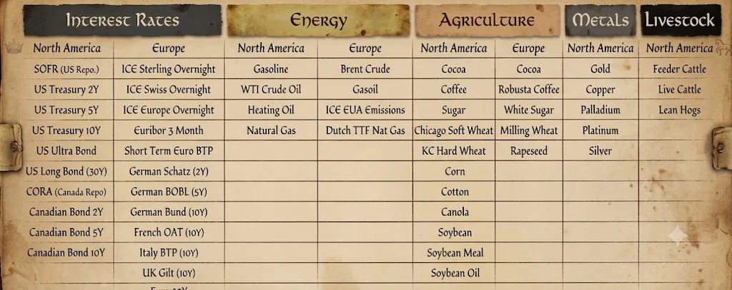
Below is the universe of exposures for its long or short positions.
Going long means making money when prices rise.
This is buying low then selling high.
Going short means making money when prices fall.
This is selling high then buying low.
It underperformed the benchmark for the quarter.
Its Q2 2026 underperformance was primarily driven by a long Brent Crude Oil position, as prices declined nearly 40% from a mid-May peak of approximately $120 per barrel to roughly $70 at quarter-end.
The Brent oil position was established in mid-March as supply constraints from the Strait of Hormuz closure drove oil prices higher. As peace talks progressed, prices reversed abruptly, making the long exposure a material drag. Strong gains through mid-May helped cushion the subsequent drawdown.
Fully Allocated Physical Gold Bullion

Historically, gold’s unique physical properties made this chemical element the premier form of commodity money.
It is chemically stable and virtually indestructible, meaning almost all gold ever mined still exists. This durability and geological rarity give gold the highest stock-to-flow ratio of any physical commodity, with annual production adding only about 1.5% to the existing supply.
This reliable scarcity protects gold from the historical debasement of other currencies, making it a superior store of value since its supply cannot easily increase as prices rise.
For our deep dive into this topic, checkout this post:

It underperformed the benchmark for the quarter.
In March 2026, gold suffered its largest absolute monthly drop since 2013.
This sharp correction was triggered by Gulf War 3 and a mix of macroeconomic shocks: an oil price spike causing US dollar scarcity, cut-off Gulf cash flows, a hawkish Fed boosting yields, and a crowded unwind of consensus longs.
These reasons are similar to why the precious metal royalty exposures sold off, which we previously wrote about.
Actively Managed Foreign Exchange (FX) Strategies
This actively managed FX strategy seeks long-term absolute returns with low/negative correlation to equities, bonds, and other alternative strategies.
FX Investing 101
Unlike retail cash exchanges that don’t earn or pay interest (like exchanging US Dollars (USD) for Mexican Pesos at the airport), institutional foreign exchange (FOREX) investing allows investors to earn a yield when buying (going long) a currency and to pay a yield when selling (going short) a currency.
For example, if you pair a short Japanese yen (JPY) yielding 2% (paying that rate) with a long Brazilian Real (BRL) yielding 13.6% (earning that rate) means you can pocket the 11.6% differential.
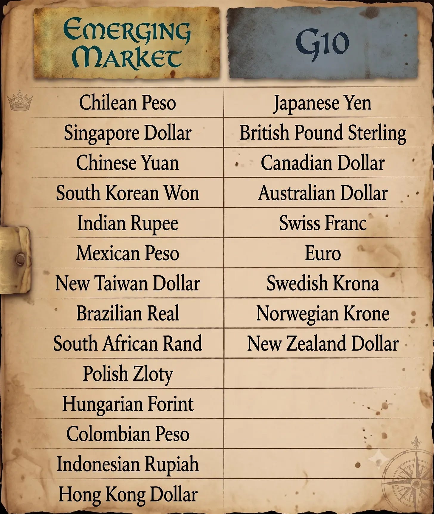
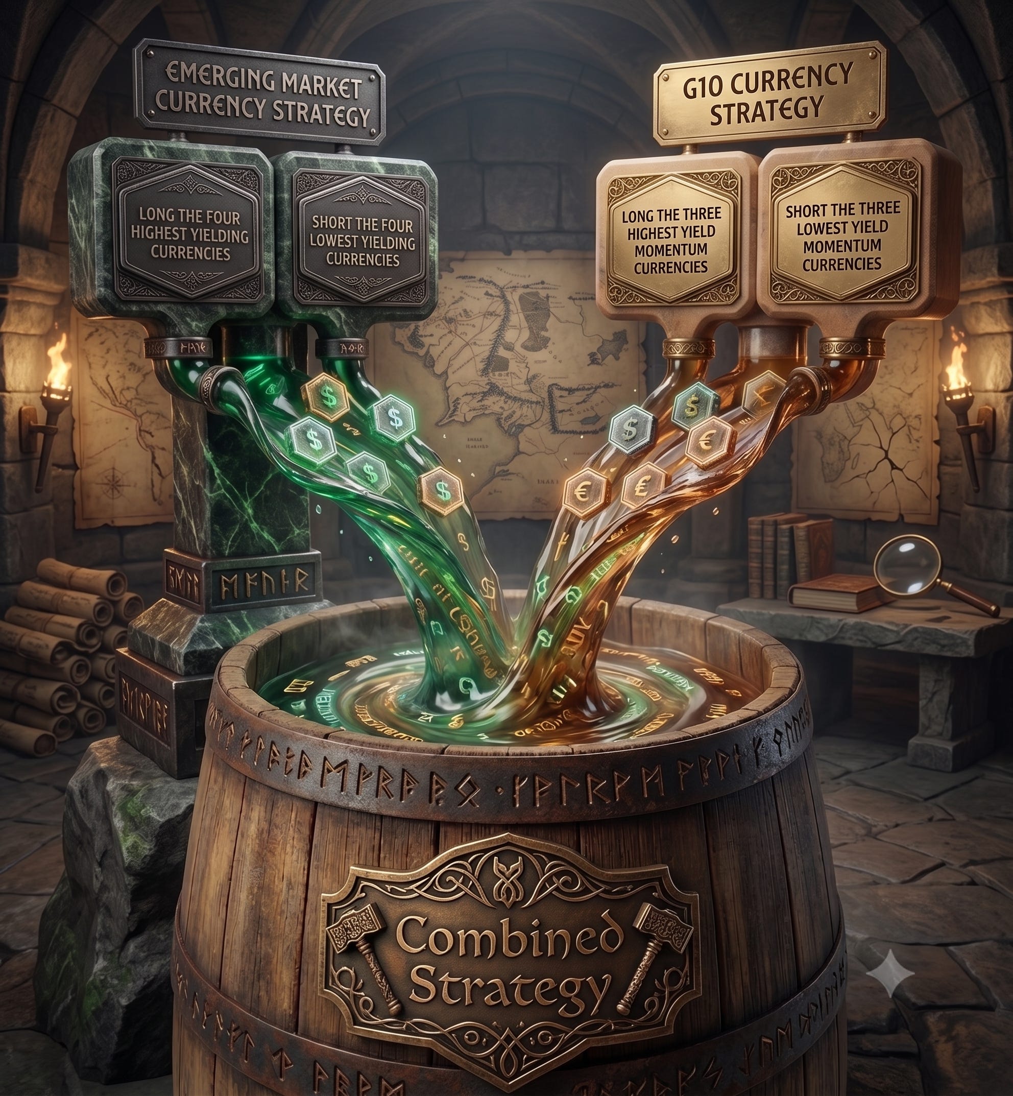
This actively managed FX strategy is a blend of two different and complimentary FX strategies: an Emerging Market FX strategy and a G10 FX strategy.
Emerging Market FX Strategy Sleeve
This strategy generates returns by capturing the “carry”—the spread between high-yielding and low-yielding currencies—by taking long positions in the most liquid highest-yielding currencies and short positions in the most liquid lowest-yielding currencies.
Weights are optimized to reduce exposure to higher volatility currencies, enhancing risk-adjusted performance due to the trend-following nature of these assets.
Critically, it is USD neutral, meaning it maintains an equal percentage of currency exposure in long and short positions relative to the USD i.e. it is NOT taking a bet on USD performance relative to other currencies.
G10 FX Strategy Sleeve
This strategy generates returns by capturing the “implied yield momentum”—the change in expectations for a currency's yield advantage over another—by taking long positions in the most liquid highest yield momentum currencies and short positions in the most liquid lowest yield momentum currencies.
Weights are optimized to reduce exposure to higher volatility currencies.
Critically, it is USD neutral, meaning it maintains an equal percentage of currency exposure in long and short positions relative to the USD i.e. it is NOT taking a bet on USD performance relative to other currencies.
Combined Strategy
When combining the EM and G10 sleeves, it weights the two sleeves inversely to the realized volatility of each sleeve.
In periods of high volatility such as during a geopolitical turmoil or a systematic financial crisis, it reduces exposure to high-volatility EM currencies, shifting focus to more stable G10 currencies.
This approach not only reduces risk but also enhances returns by capitalizing on the relative stability of the G10 currencies relative to EM.
It outperformed the benchmark for the quarter.
During the first phase of Gulf War 3, it traded sideways as high global interest rate volatility and oil price sensitivity challenged implied yields. As the war premium faded and thus volatility declined, yield signals stabilized thus the currency yield differentials regained importance.
The primary contributors to performance were from the Colombian Peso (COP), the Brazilian Real (BRL), the Hungarian Forint (HUF), and the Mexican Peso (MXN).
Defense and offense have both been important: it frequently adopted a defensive posture, holding long Japanese yen (JPY) positions as a safe haven during geopolitical tension and market volatility.
Defense
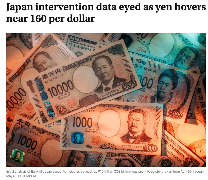
Its long JPY position is timely given the Bank of Japan’s (BoJ) rate hikes and the Ministry of Finance’s (MoF) interventions (buying JPY) to curb JPY weakness.
Additionally, its defensive strategy generated significant alpha from weaker Asian EM currencies, particularly the Korean won (KRW).
Offense
The offense also performed well, with high-yielding Latin American currencies like the Colombian Peso (COP), Brazilian Real (BRL), and Mexican Peso (MXN) posting strong gains alongside high yields. These oil-exporting currencies benefited from firm energy prices, sentiment-boosting political shifts (rightward in Colombia, slightly left in Brazil), and consistent central bank policies that anchored inflation expectations while maintaining attractive real yields.
New Positions
Actively Managed Futures Yield
This actively managed exposure seeks long-term absolute returns with low/negative correlation to equities, bonds, and other alternative strategies.
Futures yield, or “carry,” is an investment strategy that captures the embedded yield implied by an asset’s price structure, independent of market direction.
It focuses on extracting the economic benefit of holding an investment minus its holding costs.
Think of it like being a landlord.
Futures Yield or Carry is like buying a property and collecting rent. It’s the return the market may offer you for providing capital — even if prices don’t move.
In the financial markets, this “rent” or yield is the price gap between an asset’s current price (the spot price) and its price for future delivery (the futures price).
The sources of this yield represent the “cost of ownership” and vary depending on the specific asset class.
Futures Yield Example: Oil
Consider oil as an example, since this exact situation is playing out in real time during Gulf War 3.
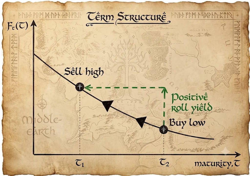
You can buy oil today (T1) at the spot price for immediate delivery (say $100).
You can buy oil today (T2) at the future price for future delivery (say $80)
This is similar to Amazon Delivery offers discounted pricing if you choose delivery within a week instead of a few hours.
A higher spot price (T1) indicates immediate delivery’s relatively scarcity, meaning one can get paid to wait for future delivery (T2).
It also encourages oil producers to quickly expand production to meet high immediate-delivery prices (T1).
If the spot price of oil remains unchanged (T1), buying oil at $80 (T2) and waiting for it to “roll” into the present $100 price (T1) earns a $20 futures yield (T2-T1).
Futures yield is our compensation for bearing the risk of what oil’s spot price (T1) will be at contract maturity.
Capturing futures yield is compensation the market is willing to pay investors for providing capital and taking on specific economic, liquidity, or credit risks from natural hedgers (like farmers, oil producers, or governments) who want to offload their price risks.
The Fundamental Reason for Futures Markets and Futures Prices
Farming is hard and planning for a farming business is difficult enough without knowing future corn prices. Therefore, farmers can “lock in” the future corn price for future delivery at future harvest time.
Because futures yield is driven by funding conditions, inventory dynamics, and pricing mechanics rather than broad economic growth or price momentum, it acts as a highly distinct return source that historically exhibits very low correlation to traditional stocks, bonds, and even other alternative strategies like trend following.
Ultimately, this actively managed futures yield strategy focuses on rent as the primary signal i.e. it buys (going long) assets that pay you to hold them and sells (going short) assets that charge you to hold them, regardless of where prices go.

Disclaimer
This website is not an offer or solicitation in any jurisdiction in which the firm is not registered. Information presented is for educational purposes only. It should not be considered specific investment advice, does not take into consideration your specific situation, and does not intend to make an offer or solicitation for the sale or purchase of any securities or investment strategies. The services, securities and financial instruments described on this website may not be suitable for you, and not all strategies are appropriate at all times. Investments involve risk and are not guaranteed. Past performance is not necessarily a guide to future performance. Independent advice should be sought in all cases.
TYME Advisors is a U.S. Securities and Exchange Commission (SEC) Registered Investment Advisor . Registration does not imply a certain level of skill or training. Information about the firm including the Customer Relationship Summary is available on the SEC’s website at www.adviserinfo.sec.gov. Information about our privacy policy is located here.